#dsa, #algorithms, #selection-algorithms, #quicksort-family, #patterns

🧠 Mind map

QuickSelect Map|700

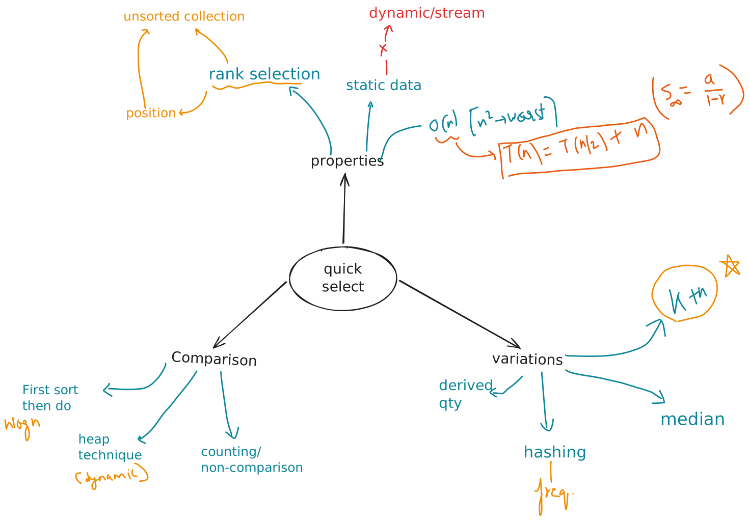
🎯 Quickselect & Selection Algorithms

**One-line definition: ** A selection algorithm finds the kth smallest/largest element (the kth order statistic) in a collection without necessarily sorting the whole thing. Quickselect is quicksort with one recursive branch amputated — partition once, then recurse into only the half that contains your target index.

🧠 The Core Insight

Quicksort’s partition step has a hidden byproduct most people never isolate: after one partition, the pivot lands in its final sorted position. Quicksort throws this fact away and recurses into both sides to fully sort. Quickselect notices that if the pivot’s final position happens to be the rank you want, you’re done — and if not, you provably only need to search one side, because the other side is guaranteed irrelevant.

🪓 “Ripped a leg off quicksort.” This is a legitimately accurate mental model, not an oversimplification. Hoare invented both quicksort (1959) and quickselect (1961) — the selection variant came as a later, separate realization, not as part of the original insight. That gap is telling: even the inventor didn’t see the amputated version immediately.

Why this isn’t “obvious in hindsight” (and that’s OK):

Sorting is normally treated as an atomic, sealed operation — cracking it open to ask “which intermediate guarantee is independently useful?” is a trained habit, not a default one.
It requires realizing you don’t need the whole sorted array — only one position to be correct. Solve exactly what’s asked, not the general problem the obvious tool produces.
Discarding a whole partition’s worth of computed work feels wasteful at first, even though it’s provably safe to discard.

Meta-pattern to carry forward: whenever you reach for a bigger/general algorithm as brute force, ask — “does this algorithm produce a smaller guarantee partway through that I could stop at?” This generates a large fraction of “aha” LeetCode mediums: quicksort → quickselect, BFS → shortest-path variants, DP → space-optimized DP, etc.

🔍 How to Identify This Pattern

Signals that a problem wants quickselect (or the selection-algorithm family broadly):

Phrasing: “kth smallest/largest,” “median,” “top K,” “K closest.”
You need one specific rank/position, not the full sorted order.
A full sort would obviously work but feels wasteful (O(n log n) when O(n) is hinted at, or n is large).
Interviewer follow-up: “can you do better than sorting?” or “what if the array doesn’t fit in memory?” (→ pushes toward heap variant).
Array is unsorted and you need an order statistic, not a search — binary search wants sorted/monotonic data; quickselect wants unsorted rank-selection.

Litmus phrasing: if the problem “smells like sort-would-obviously-work-but-is-that-necessary,” think quickselect first.

🛠️ The Generalized Template

import random

def partition(nums, left, right, pivot_index):
    pivot = nums[pivot_index]
    nums[pivot_index], nums[right] = nums[right], nums[pivot_index]  # move pivot to end
    store_index = left
    for i in range(left, right):
        if nums[i] < pivot:
            nums[store_index], nums[i] = nums[i], nums[store_index]
            store_index += 1
    nums[right], nums[store_index] = nums[store_index], nums[right]  # pivot to final place
    return store_index

def quickselect(nums, left, right, k_smallest_index):
    if left == right:
        return nums[left]

    pivot_index = random.randint(left, right)  # random pivot avoids worst-case on sorted/adversarial input
    pivot_index = partition(nums, left, right, pivot_index)

    if k_smallest_index == pivot_index:
        return nums[pivot_index]
    elif k_smallest_index < pivot_index:
        return quickselect(nums, left, pivot_index - 1, k_smallest_index)
    else:
        return quickselect(nums, pivot_index + 1, right, k_smallest_index)

def findKthSmallest(nums, k):
    return quickselect(nums, 0, len(nums) - 1, k - 1)  # k-1 = 0-indexed rank

⚠️ Details That Trip People Up

Random pivot is not optional — without it, sorted/reverse-sorted or adversarial input degrades to O(n²).
kth smallest → target index k - 1 (0-indexed rank).
kth largest → target index n - k (or negate values / flip comparator).
Mutates the input array. Copy first if mutation isn’t allowed.
Space: O(1) extra (in-place) — the interview-favorite advantage over sorting.
Convert to iterative (while left < right loop instead of recursion) if asked to avoid stack depth risk on adversarial inputs — some interviewers explicitly probe this.

🔑 Generalizing the Key

The pattern isn’t about “numbers” — it’s about partitioning by any comparable key. Compute a key, partition by that key, recurse into the relevant half. Keys seen in practice:

Distance from origin/a point (973)
Frequency count (347)
Absolute difference from a value
Any custom derived score

⏱️ Why It’s O(n) Average — Proof Sketch

Quicksort recurrence (recurses into both halves, full-width work at every level):

T(n) = 2T(n/2) + O(n)  →  O(n log n)

Quickselect recurrence (recurses into only one half):

T(n) = T(n/2) + O(n)   [average case, roughly balanced pivot]

Expanding:

T(n) = n + n/2 + n/4 + n/8 + ... + 1
     = n × (1 + 1/2 + 1/4 + ...) = n × 2 = O(n)

This is a converging geometric series — the first term (cost n) dominates the total, because every subsequent step operates on a shrinking array and decays geometrically. Quicksort’s total work does not converge this way because every level still touches the full n elements across both branches → the log n factor survives.

Formal version: with a random pivot, the pivot’s rank is uniformly distributed among the current subarray, so in expectation each partition removes a constant fraction of elements. Solving the resulting expected-value sum gives E[T(n)] = O(n) — same technique used to prove quicksort’s average-case O(n log n), but the discarded half is what kills the log factor here.

Worst case (O(n²)): a consistently bad pivot (e.g., always picking nums[left] on sorted/adversarial input) only shrinks the array by 1 element per step:

T(n) = T(n-1) + O(n) = n + (n-1) + ... + 1 = O(n²)

→ This is exactly why random pivot selection is load-bearing, not cosmetic.

🌳 Taxonomic Placement

Quickselect is a prune-and-search (decrease-and-conquer) selection algorithm — a partition-based approach to the order-statistics problem. It shares its partition primitive with quicksort and Dutch National Flag, and its pruning philosophy with binary search — used for static/batch data, swapped for heaps when data streams.

Formal category: Selection Algorithms

Algorithms that find the kth order statistic without full sorting. A named, well-studied subfield distinct from (but bordering) sorting and searching.

The Selection Algorithm Family

Algorithm	Worst case	Average case	Space	Key idea
Sort then index	O(n log n)	O(n log n)	O(n)	Brute-force baseline
Quickselect	O(n²)	O(n)	O(1)	Partition, recurse into one side
Median of Medians	O(n)	O(n)	O(1)	Deterministic good-pivot choice → guarantees worst case
Introselect	O(n log n)	O(n)	O(1)	Quickselect that falls back to median-of-medians if recursion too deep (real-world: C++ `std::nth_element`)
Heap-based selection	O(n log k)	O(n log k)	O(k)	Maintain heap of size k — good for streams
Counting/Bucket selection	O(n + range)	O(n + range)	O(range)	Bounded/small value range
Tournament method	O(n + k log n)	same	O(n)	Bracket-style, useful for small k

Closest sibling: Median of Medians. Same skeleton as quickselect, but replaces “random pivot” with “provably good pivot” (median of 5-element chunks) — trades constant-factor speed for a worst-case guarantee. Answer to “can you guarantee O(n) even in the worst case?” — know it exists and why (5-chunks guarantee the pivot avoids extreme tails), rarely need to code it live.

Direct Neighbors (same “partition-and-prune” DNA)

Binary Search — closest conceptual cousin (see dedicated comparison section below). Prunes by value comparison on sorted/monotonic data vs. quickselect’s partition position on unsorted data.
Dutch National Flag / 3-way partitioning (LC 75) — the exact same partition primitive, generalized to 3 regions (less/equal/greater) to handle duplicates. Consider this a prerequisite drill for quickselect’s partition step.
QuickSort — the parent algorithm.
Divide and Conquer, zoomed out — quickselect is D&C with an asymmetric/unbalanced split: standard D&C (merge sort, closest pair of points) recurses into both equal halves and combines; quickselect does decide-then-discard — recurse into only the surviving half. Some texts call this specific flavor “prune and search” or “decrease and conquer.”

🔗 How It Pairs With Other Patterns

Quickselect rarely appears alone in medium/hard problems — usually a subroutine inside something bigger:

Pairing	Example	Mechanism
+ Geometry (distance as key)	973. K Closest Points to Origin	Partition by squared Euclidean distance instead of raw value
+ Hashing (frequency as key)	347. Top K Frequent Elements	Hash-count frequencies first, then quickselect on frequency values
+ Greedy (median-based optimum)	462. Min Moves to Equal Array Elements II	Median is the optimal point (greedy/calculus fact); quickselect just finds it efficiently
+ Heaps (streaming swap-out)	703, 295	Quickselect doesn’t work on streaming data — re-partitioning on every insert is wasteful. This is the most important contrast pairing.
+ Construction problems	324. Wiggle Sort II	Quickselect finds median as a subroutine inside a larger array-construction algorithm

Boundary to internalize: quickselect = static/batch data. Heaps = streaming/dynamic data. Interviewers love probing this exact line (“what if numbers arrive one at a time?”).

⚔️ Quickselect vs. Binary Search on Answer

The two most-confused siblings in this family — both find “the kth/optimal value,” but they prune fundamentally differently.

	Quickselect	Binary Search on Answer
Searches over	Indices/positions in the actual array	Values in a range (may not exist in the array at all)
Needs from data	Ability to physically partition/rearrange	Ability to count/check feasibility for a guessed value
Per-step operation	Partition around a pivot (rearranges array)	Guess a value, run a monotonic feasibility/count check, shrink range
Mutates array?	Yes	No
Determinism	Randomized (needs random pivot)	Deterministic, no randomness needed
Worst-case defense	Needs median-of-medians for guaranteed O(n)	Naturally O(n log range) — no adversarial case to defend
Time	O(n) avg / O(n²) worst	O(n log(range)) typically

Mental model:

Quickselect finds where an element belongs (a position). Binary search on answer finds the smallest/largest value that satisfies a condition (a hypothesis test).

Decision Litmus Test (in order)

Single flat unsorted array, free to rearrange? → Quickselect.
Can you write count(X) = "# elements ≤ X" cheaply — especially across multiple structures (two arrays, a matrix) without rearranging? → Binary search on answer.
Is the “answer” a value that might not be an array element at all (a capacity, a time, a distance)? → Strong binary-search-on-answer signal; quickselect literally has nothing to partition.

Trigger phrase for binary search on answer: “minimize the max” / “maximize the min” framing (Koko Eating Bananas, Split Array Largest Sum, Divide Chocolate) — near-direct signature, distinct from “kth smallest” phrasing.

Worked Contrast — LC 378 (Kth Smallest in Sorted Matrix)

Quickselect approach: would require flattening the matrix into an array first — throws away the exploitable sorted-row/sorted-column structure. Wasteful.
Binary search on answer (intended): binary search over the value range [matrix[0][0], matrix[n-1][n-1]]; for guessed mid, count elements ≤ mid in O(n) via a staircase walk exploiting sorted rows/cols; shrink range based on count vs. k.
Takeaway: when input already has exploitable structure (sorted rows/cols, multiple sorted arrays), binary search on answer wins because it uses a cheap counting function instead of blind rearrangement.

Clean Drilling Pairs

Quickselect-natural	Binary-search-on-answer-natural
215. Kth Largest Element in an Array	4. Median of Two Sorted Arrays
973. K Closest Points to Origin	378. Kth Smallest Element in a Sorted Matrix
347. Top K Frequent Elements	719. Kth Smallest Pair Distance
462. Min Moves to Equal Array Elements II	410. Split Array Largest Sum
—	875. Koko Eating Bananas
—	1231. Divide Chocolate

🧰 Alternative Tools for “Find the Kth Element” (Full Tradeoff Table)

Approach	Time	Space	When to use
Sort	O(n log n)	O(1)/O(n)	k unknown in advance / need multiple ranks
Min/Max Heap of size k	O(n log k)	O(k)	Streaming data, k small, memory-constrained
Quickselect	O(n) avg	O(1)	One-shot query, array fits in memory, average-case OK
Binary Search on Answer	O(n log range)	O(1)	Cheap counting/feasibility function exists; multi-structure input
Counting sort / bucket	O(n)	O(range)	Bounded/small value range (e.g., frequencies)

Interview move: name all relevant options and justify the choice out loud, even if you ultimately code quickselect — this signals seniority more than the code itself.

📚 LeetCode Problem Bank

Must-Know Core (do first, in order)

#	Problem	Difficulty	Why	🔗
215	Kth Largest Element in an Array	Medium	Canonical quickselect problem — know both heap and quickselect solutions cold	kth-smallest-element-in-an-array
347	Top K Frequent Elements	Medium	Quickselect on frequency-as-key — very high frequency at Amazon/Meta/Google	top-k-frequent-elements-(lc-347)
973	K Closest Points to Origin	Medium	Quickselect on distance-as-key — common at Amazon (geo framing), Meta
703	Kth Largest Element in a Stream	Easy	Tests knowing when quickselect fails (streaming) → heap
295	Find Median from Data Stream	Hard	Two-heap technique; frequent follow-up to 703

Median-Specific (selection as subroutine)

#	Problem	Difficulty	Why	l🔗
462	Min Moves to Equal Array Elements II	Medium	Median via quickselect + greedy math
4	Median of Two Sorted Arrays	Hard	Binary search on partition point — classic hard bar-raiser (Google/Meta)	median-of-two-sorted-arrays
480	Sliding Window Median	Hard	Two-heap + lazy deletion, finance/trading-adjacent companies

Distance / Frequency / Custom-Key Variants

#	Problem	Difficulty	Why	🔗
692	Top K Frequent Words	Medium	Like 347 + lexicographic tie-breaking — tests comparator design	top-k-frequent-elements-(lc-347)
658	Find K Closest Elements	Medium	Binary search + two pointers is intended — good “don’t force quickselect” case	top-k-closest-elements-(lc-658)
1985	Find the Kth Largest Integer in the Array	Medium	String-number comparator edge cases, same skeleton as 215	kth-smallest-element-in-an-array
719	Find K-th Smallest Pair Distance	Hard	Binary search on answer + two pointers — common at Google	kth-smallest-pair-distance
378	Kth Smallest Element in a Sorted Matrix	Medium	Heap or binary-search-on-value; see worked contrast above	kth-smallest-element-in-a-sorted-matrix

Partition-Mechanics Practice

#	Problem	Difficulty	Why	🔗
75	Sort Colors (Dutch National Flag)	Medium	The 3-way partition primitive underlying quickselect’s partition step — very frequent standalone ask (Microsoft/Amazon)	3-Way Partitioning (Dutch National Flag)]

Deeper / Compound (top-tier bars)

#	Problem	Difficulty	Why
324	Wiggle Sort II	Medium/Hard	Median-finding (quickselect) as subroutine inside a construction problem — Google-flavored
414	Third Maximum Number	Easy	Edge-case/duplicate handling drill, low signal, occasional warm-up
767	Reorganize String	Medium	Frequency + greedy + heap, often grouped with 347’s “frequency pattern” set

Suggested Practice Sequence

Week 1 (foundational):     215 → 75 → 347 → 973
Week 1-2 (streaming):       703 → 295
Week 2-3 (compound):        462 → 378 → 658 → 1985
Week 3+ (hard bar-raisers): 4 → 719 → 324 → 480

Highest-frequency “disguised quickselect” problems in real loops: 347 and 973 — be able to code the quickselect version and explain the heap alternative + complexity tradeoffs out loud; that’s usually the real bar.

🧵 Cross-References

[[Binary Search]] — sibling pruning technique, contrast via “index-space vs. value-space” search
[[Dutch National Flag Partitioning]] — shared partition primitive
[[Heaps]] — streaming-data replacement for quickselect
[[Divide and Conquer]] — parent category; quickselect = asymmetric/decrease-and-conquer D&C
Kadane’s Algorithm, Floyd’s Cycle Detection, Boyer-Moore Majority Vote — other examples of “clever version hiding inside a brute-force algorithm’s byproduct”